
Abstract
Diabetes is a chronic disease with a high hospital readmission rate. The ability to predict readmission can greatly improve medical care. The complexity of factors and the rapid growth of healthcare data provide great opportunities for developing machine learning predictive models of hospital readmission. In this paper, we built three machine learning models using a dataset from the UCI machine learning repository: elastic-net logistic regression, random forests, and Extreme Gradient Boosting to predict readmission risk. We tuned their hyperparameters to improve their performance. We also identified important features contributing to hospital readmission. The three models had comparable performances with Area Under the Receiver Operating Characteristic (AUROC) values around 0.68. Surprisingly, the performance of all three models saturated quickly as the amount of training data grew, indicating training sizes were unlikely to be the constraining factor on the accuracy improvement. Since only a few features were identified to have influences on readmission, we think the greatest gains in predictive performance of hospital readmission will derive from improved feature selection and representation.
Introduction
Diabetes is a chronic disease caused by high levels of blood sugar ((CDC, “What is Diabetes?,” Centers for Disease Control and Prevention, Jul. 07, 2022. https://www.cdc.gov/diabetes/basics/diabetes.html (accessed Nov. 06, 2022).)). Common symptoms of diabetes include but are not limited to being unusually thirsty or hungry, having a need to urinate alot, unexplained loss of weight, mood swings, and feeling tired and weak ((CDC, “Diabetes Symptoms,” Centers for Disease Control and Prevention, Mar. 02, 2022. https://www.cdc.gov/diabetes/basics/symptoms.html (accessed Nov. 06, 2022).)). The body’s inability to gain energy from glucose greatly decreases the effectiveness of the immune system, making it much more susceptible to infections ((A. Berbudi, N. Rahmadika, A. I. Tjahjadi, and R. Ruslami, “Type 2 Diabetes and its Impact on the Immune System,” Curr Diabetes Rev, vol. 16, no. 5, pp. 442–449, 2020, doi: 10.2174/1573399815666191024085838.)). The most recent report from the Centers for Disease Control and Prevention estimates that approximately 11.3% of people in the United States (37.3 million people), suffer from diabetes ((“National Diabetes Statistics Report | Diabetes | CDC,” Jan. 20, 2022. https://www.cdc.gov/diabetes/data/statistics-report/index.html (accessed Aug. 28, 2022).)).
Like other chronic diseases, such as heart conditions, diabetes is associated with higher chances of hospital readmission. According to an article published in 2017, “Thirty-day readmission rates for hospitalized patients with [diabetes] are reported to be between 14.4 and 22.7%, much higher than the rate for all hospitalized patients (8.5–13.5%)” ((S. Ostling et al., “The relationship between diabetes mellitus and 30-day readmission rates,” Clin. Diabetes Endocrinol., vol. 3, p. 3, 2017, doi: 10.1186/s40842-016-0040-x.)).
The main indicator used to measure the effectiveness of care is the hospital’s 30-day readmission rate ((C. Fischer, H. F. Lingsma, P. J. Marang-van de Mheen, D. S. Kringos, N. S. Klazinga, and E. W. Steyerberg, “Is the Readmission Rate a Valid Quality Indicator? A Review of the Evidence,” PLoS One, vol. 9, no. 11, p. e112282, Nov. 2014, doi: 10.1371/journal.pone.0112282.)). Hospitals are penalized by Medicare for increased rates ((U. Winblad, V. Mor, J. P. McHugh, and M. Rahman, “ACO-Affiliated Hospitals Reduced Rehospitalizations From Skilled Nursing Facilities Faster Than Other Hospitals,” Health Aff. Proj. Hope, vol. 36, no. 1, pp. 67–73, Jan. 2017, doi: 10.1377/hlthaff.2016.0759.)) and patients choose hospitals with low readmission rates ((C. K. McIlvennan, Z. J. Eapen, and L. A. Allen, “Hospital Readmissions Reduction Program,” Circulation, vol. 131, no. 20, pp. 1796–1803, May 2015, doi: 10.1161/CIRCULATIONAHA.114.010270.)), incentivizing hospitals to decrease their readmission. The ability to predict readmission and identify risk factors will increase hospitals’ adherence to Medicare guidelines, improve the quality of patient care, and reduce the costs of healthcare ((S. Upadhyay, A. L. Stephenson, and D. G. Smith, “Readmission Rates and Their Impact on Hospital Financial Performance: A Study of Washington Hospitals,” Inquiry, vol. 56, p. 0046958019860386, Jul. 2019, doi: 10.1177/0046958019860386.)).
Dozens of factors can affect the probability of readmission for a patient, such as diagnosis, time spent in the hospital, what treatments they received, etc. The heterogeneity and complexity of those factors makes it extremely difficult to identify key factors and predict readmission risk. Researchers would have to go through hundreds of thousands of data points, each with dozens of features in order to find a method to correctly predict readmission of a patient. The difficulty makes machine learning a very viable option for creating a model.
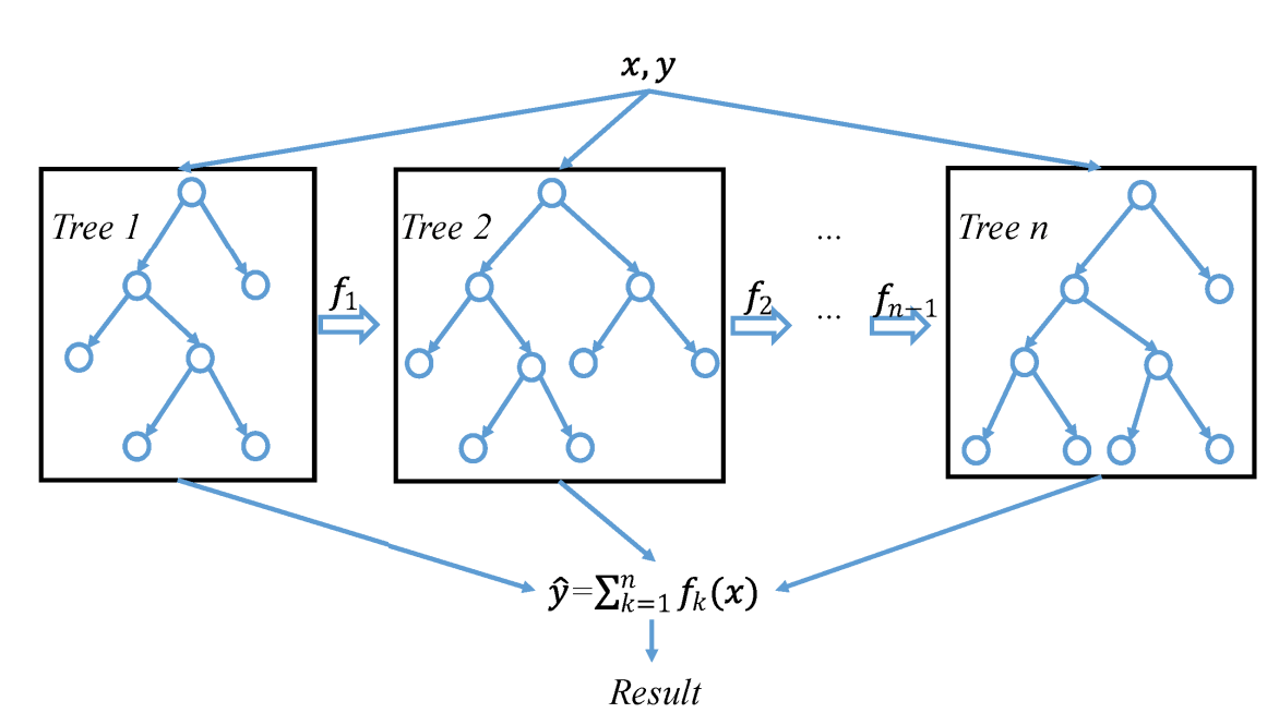
One model that can handle large datasets with good predictive ability is gradient boosting. Gradient boosting, first proposed by Jerome H. Friedman in 1999, improved on previous machine learning models by constructing additive models from fitting a base learner to current residuals by minimizing the least squares. Each iteration of the training data for the base learner is a subset of data points randomly drawn without replacement from the full training data. This improves the accuracy, training speed, and gives the model greater resilience from overfitting ((J. H. Friedman, “Greedy function approximation: A gradient boosting machine.,” Ann. Stat., vol. 29, no. 5, pp. 1189–1232, Oct. 2001, doi: 10.1214/aos/1013203451.)).
Extreme Gradient Boosting (XGBoost), was developed in 2014 by Tianqi Chen and Carlos Guestrin ((T. Chen and C. Guestrin, “XGBoost: A Scalable Tree Boosting System,” in Proceedings of the 22nd ACM SIGKDD International Conference on Knowledge Discovery and Data Mining, New York, NY, USA, Aug. 2016, pp. 785–794. doi: 10.1145/2939672.2939785.)). XGBoost’s main differences from regular Gradient boosting includes using second order partial derivatives in order to find the optimal reduction in the loss function quicker and more accurately, and also using advanced regularization in L1 and L2 weights, reducing the variance of the model ((A. Natekin and A. Knoll, “Gradient boosting machines, a tutorial,” Front. Neurorobotics, vol. 7, 2013, Accessed: Aug. 28, 2022. [Online]. Available: https://www.frontiersin.org/articles/10.3389/fnbot.2013.00021)).
XGBoost has been successfully applied to recent classification problems, such as insurance claim predictions ((M. A. Fauzan and H. Murfi, “The accuracy of XGBoost for insurance claim prediction,” Int. J. Adv. Soft Comput. Its Appl., vol. 10, no. 2, pp. 159–171, 2018.)). It has also been applied in the medical domain, for example to diagnose chronic kidney disease ((A. Ogunleye and Q.-G. Wang, “XGBoost Model for Chronic Kidney Disease Diagnosis,” IEEE/ACM Trans. Comput. Biol. Bioinform., vol. 17, no. 6, pp. 2131–2140, Dec. 2020, doi: 10.1109/TCBB.2019.2911071.)). XGBoost, however, has not been extensively used to predict hospital readmission in patients with chronic diabetes or identify the most influential factors for patient readmission.
Previous studies have trained different machine learning based classifiers to predict hospital readmission for patients diagnosed with a variety of diseases. A comprehensive review summarized that of 59 trained machine learning models, 23 were tree-based methods, 14 were neural network models, 12 were regularized logistic regression, and 10 were support vector machine models. Of those models, the median AUROC was 0.68 with an IQR of 0.64-0.76 ((D. Kansagara et al., “Risk prediction models for hospital readmission: a systematic review,” JAMA, vol. 306, no. 15, pp. 1688–1698, Oct. 2011, doi: 10.1001/jama.2011.1515.)). Different machine learning-based methods showed different performances. For example, a machine learning-based model achieved better performance in predicting patient readmission with heart failure than a simple logistic regression model ((B. J. Mortazavi et al., “Analysis of Machine Learning Techniques for Heart Failure Readmissions,” Circ. Cardiovasc. Qual. Outcomes, vol. 9, no. 6, pp. 629–640, Nov. 2016, doi: 10.1161/CIRCOUTCOMES.116.003039.)). XGBoost achieved a higher AUROC value than logistic regression for predicting 90-day readmissions in patients with Ischemic Stroke ((Y. Xu et al., “Extreme Gradient Boosting Model Has a Better Performance in Predicting the Risk of 90-Day Readmissions in Patients with Ischaemic Stroke,” J. Stroke Cerebrovasc. Dis. Off. J. Natl. Stroke Assoc., vol. 28, no. 12, p. 104441, Dec. 2019, doi: 10.1016/j.jstrokecerebrovasdis.2019.104441.)) and had an AUROC of 0.738 for predicting patient readmission with mental or substance use disorders ((D. Morel, K. C. Yu, A. Liu-Ferrara, A. J. Caceres-Suriel, S. G. Kurtz, and Y. P. Tabak, “Predicting hospital readmission in patients with mental or substance use disorders: A machine learning approach,” Int. J. Med. Inf., vol. 139, p. 104136, Jul. 2020, doi: 10.1016/j.ijmedinf.2020.104136.)).
Although machine learning classifiers have been developed to predict readmission for a variety of diseases, studies on modeling readmission risk for diabetic patients are very limited. In this paper, we used a dataset from the UCI machine learning repository (Methodology) to train three models: elastic-net logistic regression, random forests, and XGBoost to predict readmission risk and estimate the importance of features. The AUROC scores of logistic regression, random forests, and XGBoost models were 0.6722, 0.6802, and 0.6812, respectively. Surprisingly, the performance of all three models saturated quickly as the amount of training data grew. Diagnosis, specific admission sources (such as an emergency), and the use of diabetes medications were identified as main factors influencing readmission in diabetic patients.
Results
Table 1 lists the mean and standard deviation of accuracy (ACC), AUROC, and area under precision-recall curve (AUPRC) of the logistic regression, random forest, and XGBoost models with optimal parameters tuned by Halving Random Search method.
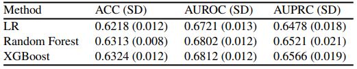
As expected, XGBoost achieved the highest accuracy, AUROC, and AUPRC scores. However, there was no significant difference in the performance between XGBoost and random forest. The superiority of XGBoost and random forest over logistic regression appeared to be subtle, but the three performance metrics of the XGBoost and random forest model were exceeding two standard deviations higher than the performance metrics of the elastic net logistic regression model. The performance of the XGBoost model compared to the random forest model is harder to interpret, as the performance metrics were all within two standard deviations of each other. All three models had low standard deviation, suggesting they all had stable performance. This meant that hyperparameter (Methodology: Hyperparameters) tuning successfully reduced overfitting, as overfitting leads to a larger standard deviation of the performance during cross-validation..
We have also plotted the distribution of the weights of features in the logistic regression model (Figure 1). Figure 2 are the top five features of the logistic regression model viewed as the most increasing and top five features viewed as most decreasing of patient readmission risk. Investigating the distribution of the weights (Fig. 1), we found most features had weights around zero, suggesting that L1 regularization deemed them useless to predicting hospital readmission.
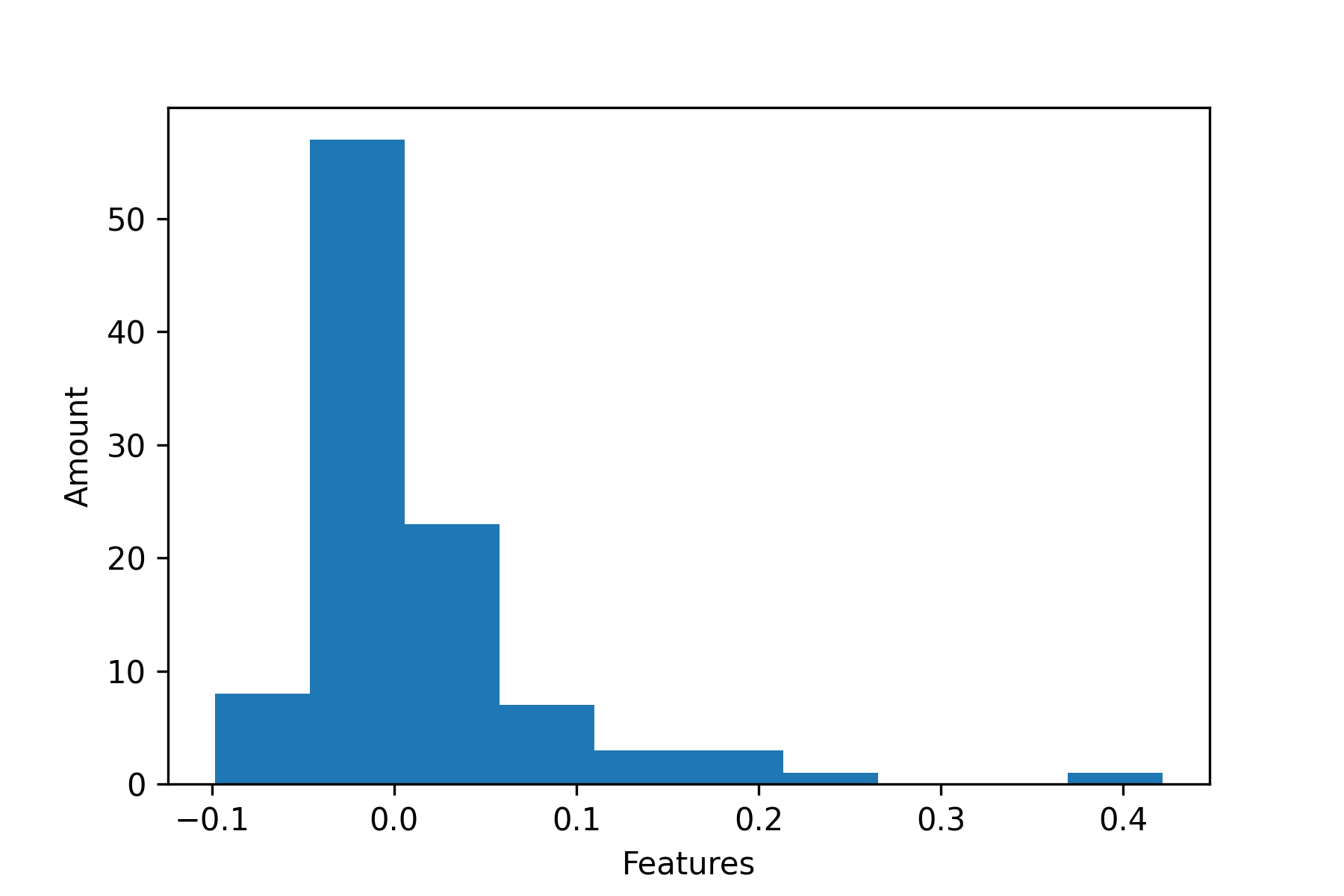
Figure 1 | Distribution of feature weights
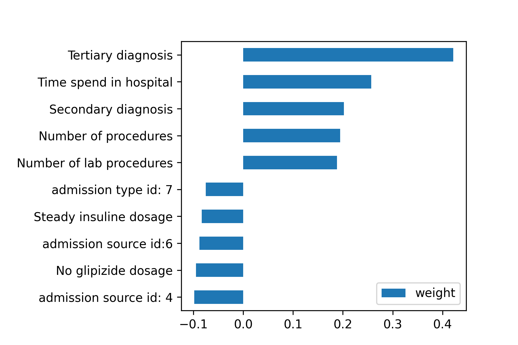
Note that the primary, secondary, and tertiary diagnosis features were their target encoded values. The features charge disposition id, admission source id, and admission type id are explained in the IDs_mapping table that is included when downloading the data set. For the IDs on Figure 2, admission type id: 7, admission source id: 6, and admission source id: 4 corresponds to “trauma center”, “transfer from another health care facility”, and “transfer from a hospital,” respectively.
The importance of the features in the XGboost models were measured in their cover as defined in the Methodology section. The distribution of the feature cover score is shown in Figure 3, and the bar graph of the ten features with the highest cover is shown in Figure 8.

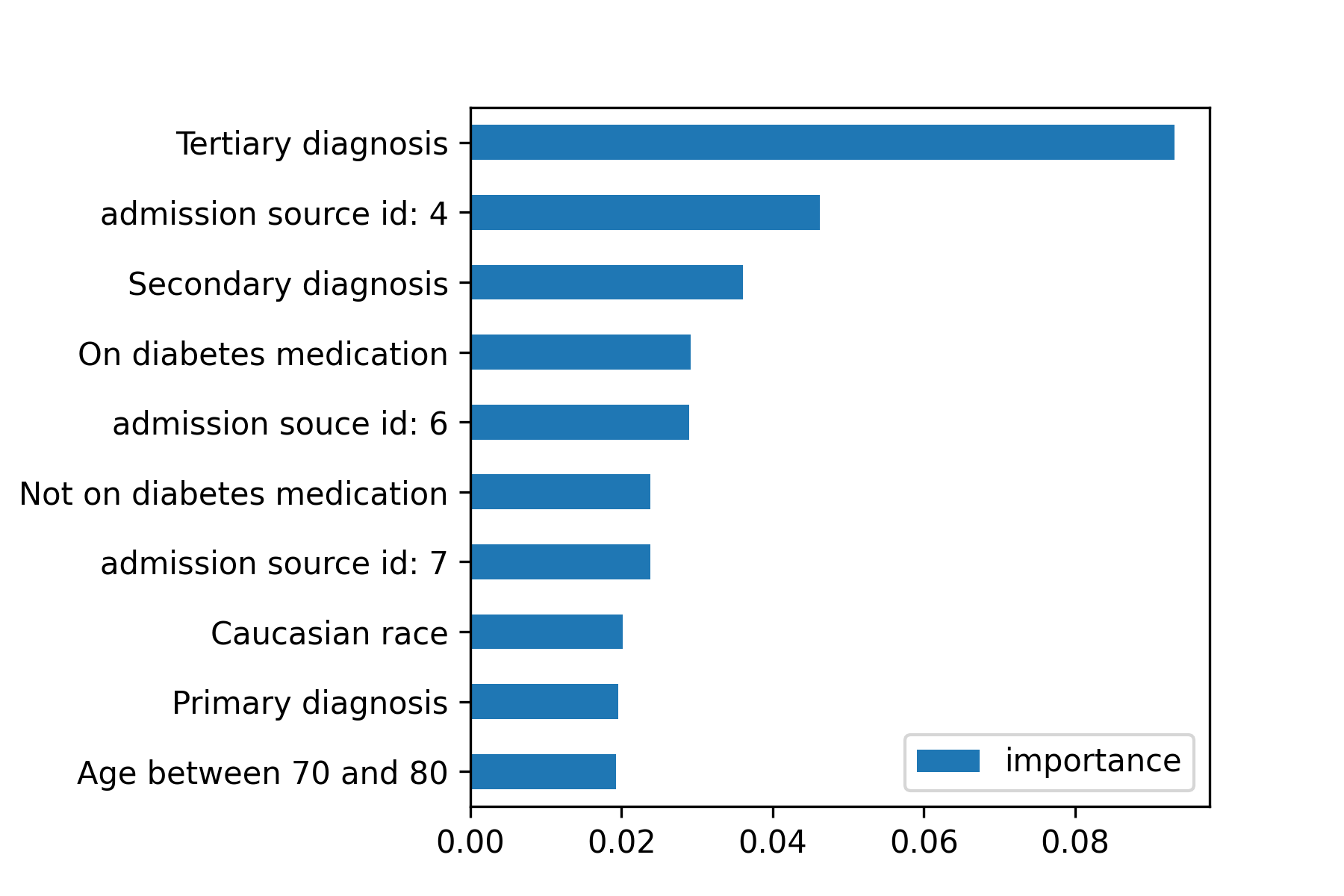
Like the results from the logistic regression model, features charge disposition id, admission source id, and admission type id are explained in the IDs_mapping table. For the IDs on Figure 9, admission source id 7, 6 and 4 corresponds to “emergency room”, “transfer from another health care facility”, and “transfer from a hospital,” respectively.
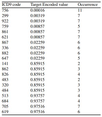
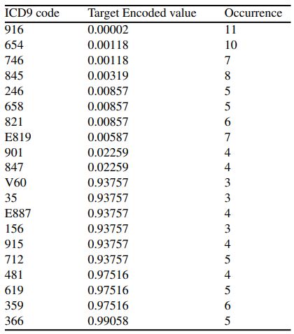
In order to interpret the importance of the three diagnosis features, we plotted the target encoded value versus the frequency of each ICD9 diagnosis of primary, secondary, and tertiary diagnosis in Figure 5, Figure 6, and Figure 7, respectively. Note that a target encoded value >0.5 indicates a positive correlation and vice versa.
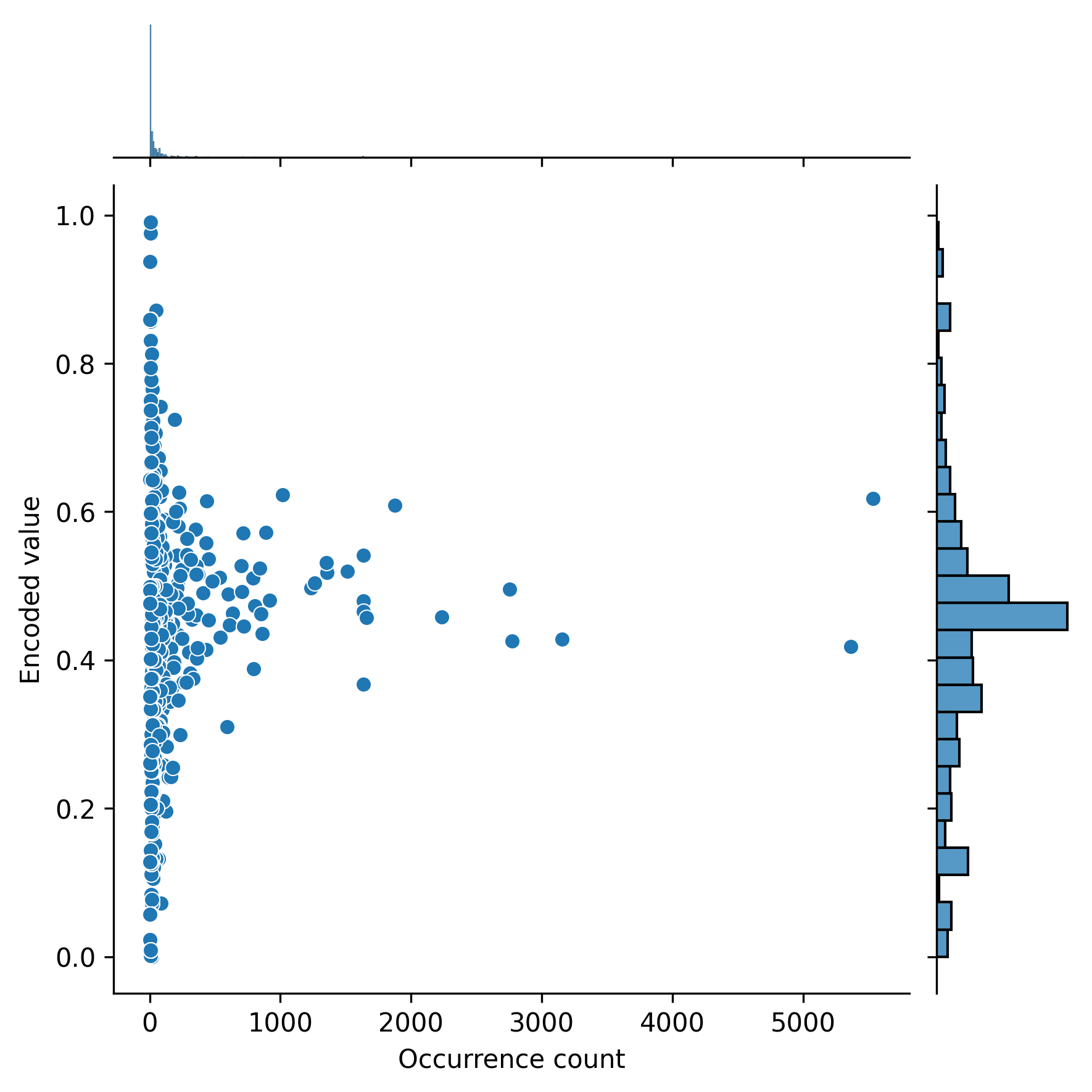
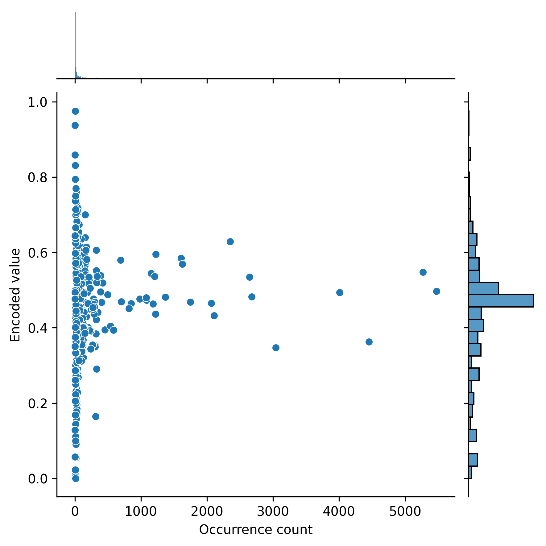
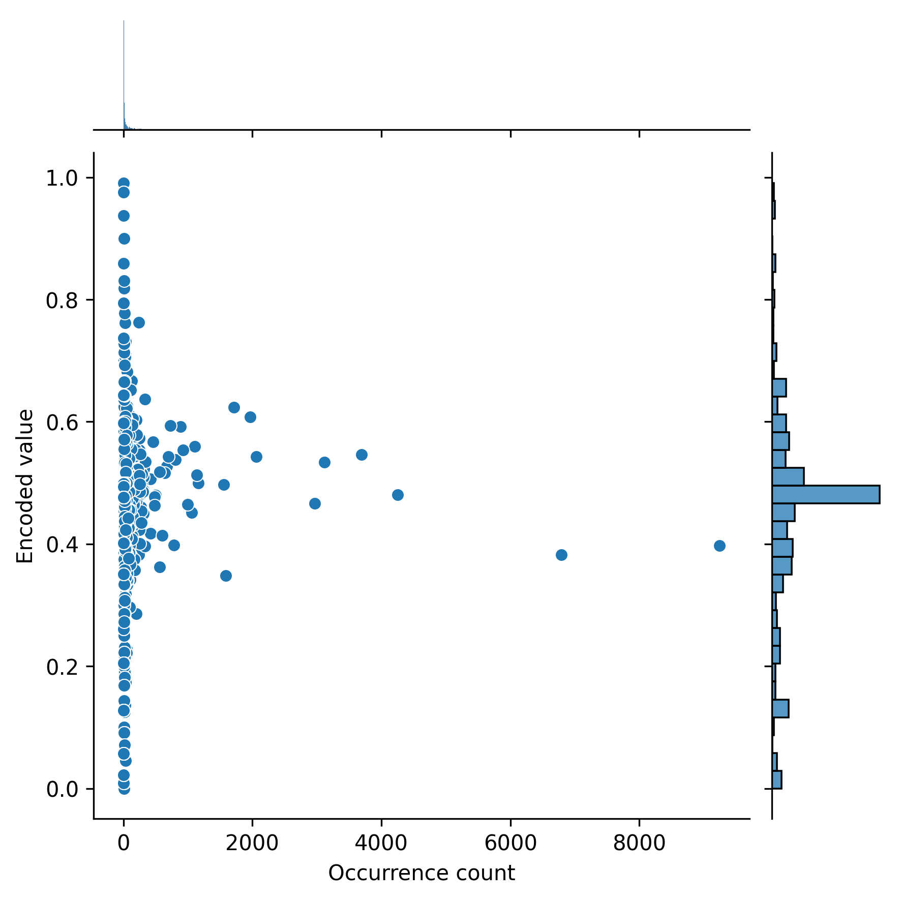
The diagnosis that each code corresponds to can be found in the ICD9 book ((World Health Organization, “International classification of diseases?: [9th] ninth revision, basic tabulation list with alphabetic index,” World Health Organization, 1978. Accessed: Aug. 30, 2022. [Online]. Available: https://apps.who.int/iris/handle/10665/39473)).
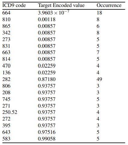
We also listed the ten ICD9 codes with the highest and ten ICD9 codes with the lowest target encoded values and their occurrence for primary, secondary, and tertiary diagnoses in tables 2, 3, and 4, respectively.
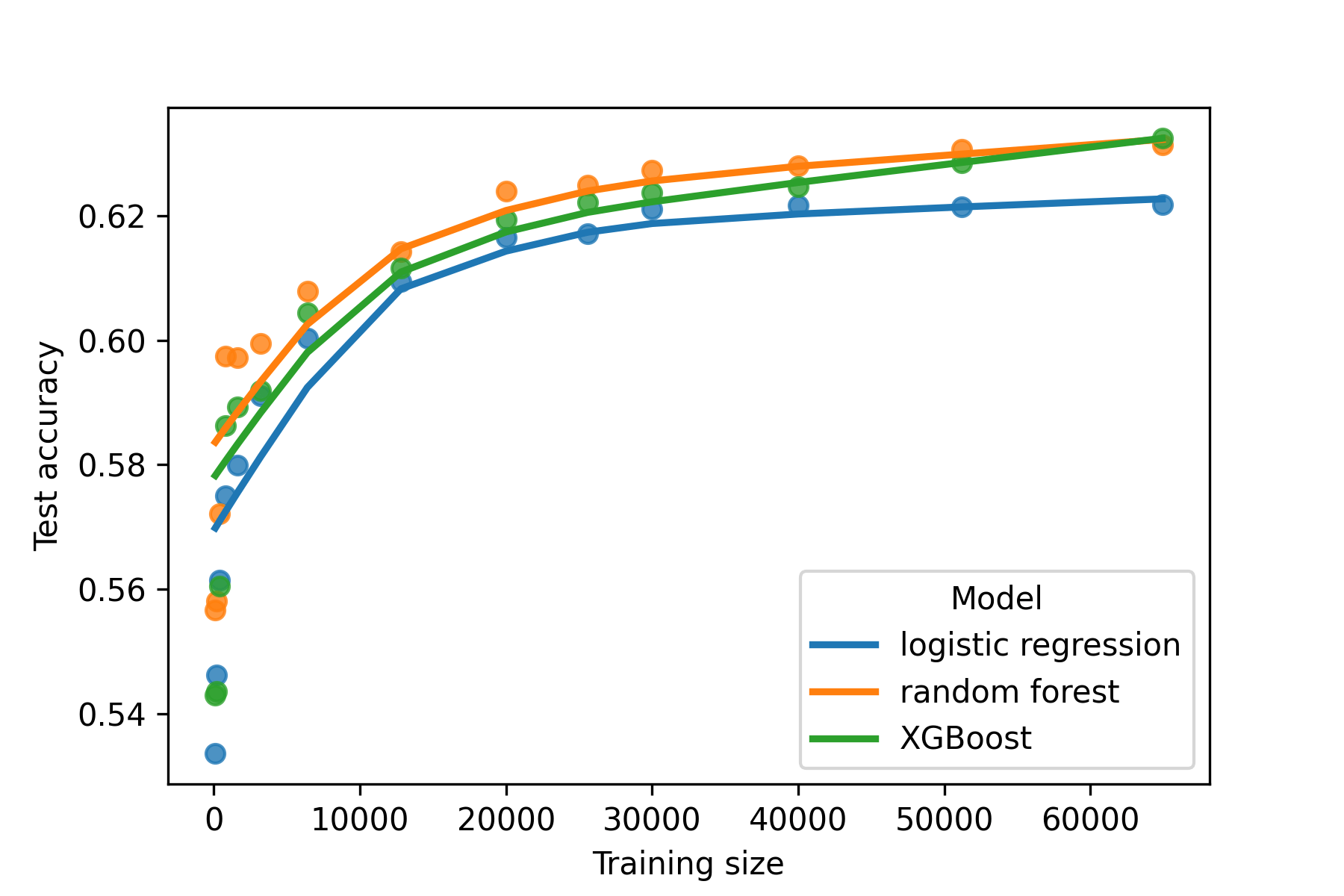
Finally, we investigated whether existing models will continue to improve as data grows, or saturate in performance (Figure 8). We found that the effect of additional training samples is diminished as the data grows, especially after reaching 20,000 subjects.
Discussion
In this study, we built three machine learning models, logistic regression with elastic net penalty, random forest, and XGBoost to predict hospital readmission of patients with diabetes. Although the XGBoost model achieved the highest AUROC score, its improvement over the logistic regression and random forest was modest and none of the models had an AUROC score exceeding 0.7. The accuracy increases also plateaued at the full dataset size, indicating a larger training set would be unlikely to improve accuracy.
The fact that model performance plateaued at less than 0.7 AUROC suggests that the dataset suffered from label noise or insufficient predictive features. The distribution of weights for the logistic regression model and cover scores for the XGBoost model also showed that most of the features had close to zero value for predicting hospital readmission. Furthermore, even though ICD-9 codes were among the most important features, the most frequent primary, secondary, and tertiary diagnoses were encoded with uninformative values close to the baseline value of 0.476. This is the proportion of patients in the dataset that were readmitted, which suggests that, in isolation, the vast majority of ICD-9 codes were not informative for predicting readmission.
Actionable insights may be derived from the most important features identified in this study. For example, patients that were assigned ICD-9 codes with high target encoded values may be important to study in case review. Future work may improve the insights derived from these models as well. While ICD-9 codes with a relatively high or low target encoding (Methodology: Categorical Encoding and Scaling) were rare, limiting the impact of reviewing these cases with these codes, ICD9 codes can also be embedded ((Y. Choi, C. Y.-I. Chiu, and D. Sontag, “Learning Low-Dimensional Representations of Medical Concepts,” AMIA Summits Transl. Sci. Proc., vol. 2016, pp. 41–50, Jul. 2016.)). This creates a continuous representation of codes such that codes with similar embeddings can all be flags for case review. Using embeddings would also circumvent limitations of target encodings, which prevent models from extrapolating to unseen diagnosis. However, using ICD-9 codes as a predictive feature has inherent limitations. ICD-9 codes are used for billing and are generally recorded after a patient is discharged, any model trained on this dataset is only useful for retrospective studies and applications.
Based on this study, we hypothesize that the greatest gains in predictive performance for hospital readmission will not improve with more data points, but will rather require new features to be collected to reduce label noise and continuous embeddings of diagnostic codes to improve generalizability. This will help fill the need for models that explicitly incorporate clinically actionable data and define and identify potentially preventable readmissions, which is critical for reducing readmission in diabetic patients and to triage them for case review and potential interventions.
Methodology
Data set acquisition and cleaning
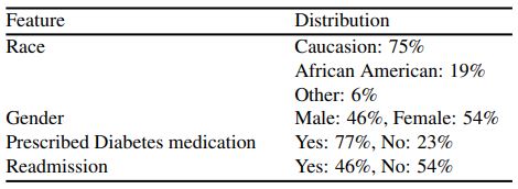
The dataset was downloaded from the UCI machine learning repository. It consisted of 101,766 diabetic patients and 50 features collected over 10 years (1998-2008) in 130 US hospitals ((B. Strack et al., “Impact of HbA1c Measurement on Hospital Readmission Rates: Analysis of 70,000 Clinical Database Patient Records,” BioMed Res. Int., vol. 2014, p. e781670, Apr. 2014, doi: 10.1155/2014/781670.)). Of those features, one was the target variable-readmission, two were encounter ID and patient number, and 47 were variables covering a multitude of clinical and sociodemographic information, such as ICD-9 diagnosis, the length of hospital stay, admission source, discharge location, age, sex, and race. The readmission outcome had three categories, NO if the patient was not readmitted, <30 if the patient was readmitted in less than 30 days, and >30 if the patient was admitted in more than 30 days. Table 5 shows the statistics of some of the features in the dataset.
We first cleaned the data by removing variables with a large portion of missing data, including weight, payer code, and medical specialty (97%, 52%, and 53% of missing data, respectively). Glucose serum and Alc test result columns were also dropped because most of the patients were not tested. We removed the patients who would clearly not be readmitted, e.g., patients expired or were discharged to hospice. Furthermore, we dropped data points with an unknown feature. After data cleaning, there were 81,143 data points each with 42 features. We then split the data set into training and test sets in a 80-20 stratified split since the readmission outcome was slightly imbalanced with 52.4% of no readmission.
Categorical Encoding and Scaling
For the readmission outcome, “NO” was encoded by 0, and <30 and >30 were combined and encoded by 1, which showed the connection between the two outcomes and allowed for target encoding. Since machine learning models can only use quantitative inputs, categorical variables with low cardinality (all categorical features except diagnosis 1, diagnosis 2, and diagnosis 3) were converted into quantitative features through one-hot encoding (The first column for each feature was dropped for the elastic-net Logistic Regression model). The diagnosis 1, diagnosis 2, and diagnosis 3 features each had over 700 unique International Classification of Diseases Ninth Revision (ICD9) ((World Health Organization, “International classification of diseases?: [9th] ninth revision, basic tabulation list with alphabetic index,” World Health Organization, 1978. Accessed: Aug. 30, 2022. [Online]. Available: https://apps.who.int/iris/handle/10665/39473)) values. One-hot encoding of those diagnoses would result in a training data set over 20 times larger than one without encoding, leading to over 20 times longer training time. Therefore, these three diagnoses were encoded through target encoding ((“Target Encoder — Category Encoders 2.5.0 documentation.” https://contrib.scikit-learn.org/category_encoders/targetencoder.html (accessed Sep. 04, 2022).)), where the features were replaced by their probability of the target value and the prior probability of the target for the whole the training data. The data sets then went through standard scaling [z=(x-?)/?], where ? is the mean and ? is the standard deviation. The standard scaling ensured fast training and comparable weights of each feature.
Categorical encoder and standard scaling were applied to the training and test data sets through a pipeline (Fig 9.), ensuring that the target encoder and standard scaling was fit to the training data set, preventing data leakage.

Machine Learning Models
We applied three Machine Learning models for classification, logistic regression with elastic net penalty, Random Forest, XGBoost.
Elastic Net Logistic Regression
The logistic function was invented in the 19th century by Pierre François Verhulst in order to describe population growth ((J. S. Cramer, “The Origins of Logistic Regression.” Rochester, NY, Dec. 01, 2002. doi: 10.2139/ssrn.360300.)). The logistic regression model uses the sigmoid activation function, similar to the graph of a population shown by Verhulst, and bounds the output between 0 and 1. The value from the sigmoid function is the probability of the event being 1. The threshold to determine the prediction was set to the base parameter of 0.5. The threshold balances type I and type II errors. Increasing the threshold reduces type I errors but raises type II errors, and vice versa ((A. Banerjee, U. B. Chitnis, S. L. Jadhav, J. S. Bhawalkar, and S. Chaudhury, “Hypothesis testing, type I and type II errors,” Ind. Psychiatry J., vol. 18, no. 2, pp. 127–131, Jul. 2009, doi: 10.4103/0972-6748.62274.)).
Logistic regression models are straightforward to implement and interpret. The straightforwardness comes from the fact that the training process is to assign weights to each independent variable, which are summed and fed into the activation function (sigmoid). Weights are trained to minimize the prediction error, which is the difference between the predicted probability and the actual result. The weights reflect the importance of each independent feature to the dependent variable, which is hospital readmission in this case. The logistic model used in this study was regularized by L1 and L2 regularization. L2 penalizes the sum of the square of the weights, while L1 penalizes the sum of the absolute value of the weights. L2 penalizes large weights, while L1 reduces weights towards 0, forming sparse models. An elastic-net model uses both L1 and L2 regularization to reduce overfitting.
Random Forest
Random forest was introduced in 2001 by Leo Bremian, a distinguished statistician of University of California, Berkeley ((L. Breiman, “Random Forests,” Mach. Learn., vol. 45, no. 1, pp. 5–32, Oct. 2001, doi: 10.1023/A:1010933404324.)). Random forest is an ensemble method for regression and classification by constructing an uncorrelated forest of decision trees. Each individual tree is built from sampling rows of training data with replacement and feature randomness. Random forest is an extension of the bagging method ((L. Breiman, “Bagging predictors,” Mach. Learn., vol. 24, no. 2, pp. 123–140, Aug. 1996, doi: 10.1007/BF00058655.)), consisting of a random sample of training data with replacement and the combination of outputs .
The random forest model has many advantages over the decision tree model ((P. T R, “A Comparative Study on Decision Tree and Random Forest Using R Tool,” IJARCCE, pp. 196–199, Jan. 2015, doi: 10.17148/IJARCCE.2015.4142.)). The random forests model creates a large number of relatively uncorrelated trees as only a subset of features and subjects are considered while building each individual tree, reducing the chance of over reliance on a few data points or features. The random forest model is also stabler as its final output comes from each individual tree “voting” on the outcome instead of just from one tree.
Extreme Gradient Boosting
XGBoost was another ensemble method used in this study. Boosting is the other common ensemble technique ((R. E. Schapire, “A brief introduction to boosting,” in Proceedings of the 16th international joint conference on Artificial intelligence – Volume 2, San Francisco, CA, USA, Jul. 1999, pp. 1401–1406.)), and trains each tree simultaneously and independently, while boosting trains each tree in a sequential order to correct the error of the previous tree.
Gradient boosting uses boosting to construct additive models from fitting a base learner to current residuals by minimizing the least squares. Each iteration of the training data for the base learner is sampled without replacement from the full training data. XGBoost, built from regular gradient boosting, uses second partial derivatives in order to find the optimal reduction of the loss function, and also uses advanced L1 and L2 regularization, making it less susceptible to overfitting.
Hyperparameters
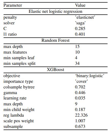
We used scikit-learn to build the elastic net logistic regression model and the random forest ((L. Buitinck et al., “API design for machine learning software: Experiences from the scikit-learn project,” API Des. Mach. Learn. Softw. Exp. Scikit-Learn Proj., Sep. 2013.)) and the XGBoost package from its namesake model ((“XGBoost Documentation — xgboost 1.6.2 documentation.” https://xgboost.readthedocs.io/en/stable/index.html (accessed Sep. 02, 2022).)). We described how we chose and tuned specific parameters in this section. Default values were used for unmentioned parameters. The detailed descriptions of the parameters of elastic net and logistic regression are found on scikit-learn and each parameter for were listed in XGBoost documentation ((“XGBoost Parameters — xgboost 1.6.2 documentation.” https://xgboost.readthedocs.io/en/stable/parameter.html (accessed Sep. 02, 2022).))
The hyperparameters were tuned using scikit-learn’s Halving Random Search method ((“sklearn.model_selection.HalvingRandomSearchCV,” scikit-learn. https://scikit-learn/stable/modules/generated/sklearn.model_selection.HalvingRandomSearchCV.html (accessed Sep. 02, 2022).)). The hyperparameters were generated by the uniform function when a float was required, and a random integer function when an integer was in need. The range of the generator would shift slightly if the best performing model’s parameter was near the boundary. Halving random search differs from random search because it first trained models with fewer resources, e.g., fewer samples. The sets of model parameters yielding accuracy in the bottom two-thirds were eliminated, while the rest passed on to the next iteration to repeat the process, except the resources used were doubled. This process repeated until only one set of parameters was left, which was then selected. The accuracy was computed from two-fold cross validation. The use of fewer resources in the iterations allowed Halving Random Search to evaluate a much larger combination of parameters in the same duration as random search, making more efficient discovery of optimal parameters.
Table 6 shows the models and their respective parameter settings. Bolded parameters were tuned, while other parameters were different from the default, but not tuned. Unmentioned parameters were left as their default values. Note that the random_state parameter of all of the models were set to 0 for reproducibility.
Performance and Interpretation
Model performance was assessed by three metrics: accuracy, area under receiver operating characteristic (AUROC), and area under precision-recall curve (AUPRC). The testing set was split into five folds to estimate standard deviation of the three metrics. For the XGBoost model, the importance of each feature came from their cover. Cover is calculated using predictions at that point in the tree, and the 2nd derivative with respect to the loss function. The cover of a feature is the average cover in all of the splits where the feature is used.
We also analyzed how the sample size of the training data affected the accuracy by fitting models with varying amounts of training data (a geometric sequence starting with 100 increasing by factors of 2 until 51,200, also 20,000, 30,000, and 40,000 to fill in gaps, and the final one where the entire training set was used).


